")
")
1D composite wall with internal heat generation and convection
System
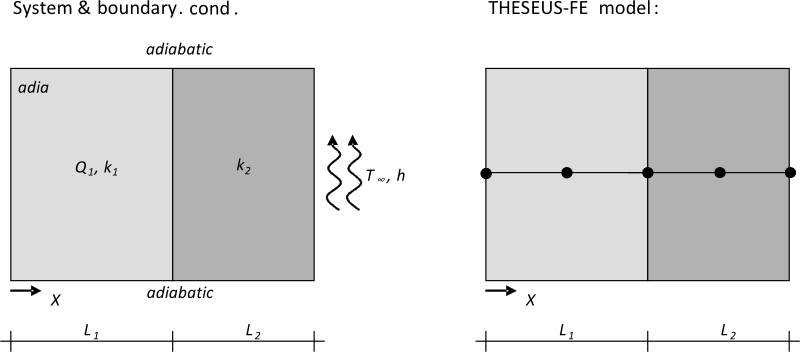
System and boundary conditions
| Quantity | Value | Units | Description |
|---|---|---|---|
| Q 1 | 1.5E6 | W / m 3 | Heat generation |
| k 1 | 75 | W / m*K | Conductivity in left layer |
| L 1 | 0.05 | m | Thickness of left layer |
| k 2 | 150 | W / m*K | Conductivity in right layer |
| L 2 | 0.02 | m | Thickness of right layer |
| h | 1000 | W / m 2 *K | Convective heat transfer coefficient |
| T ∞ | 30 | °C | Ambient temperature |
Problem description
A two layer composite wall with heat generation in the first layer is modelled. The composite wall is adiabatic on one side and has convection boundary condition on the other. The exact analytic solution for the temperature distribution is given in [1].
THESEUS‑FE model
1 quad shell element (PSHELL3) with 2 layer and 6 discretization points per layer.
Comment
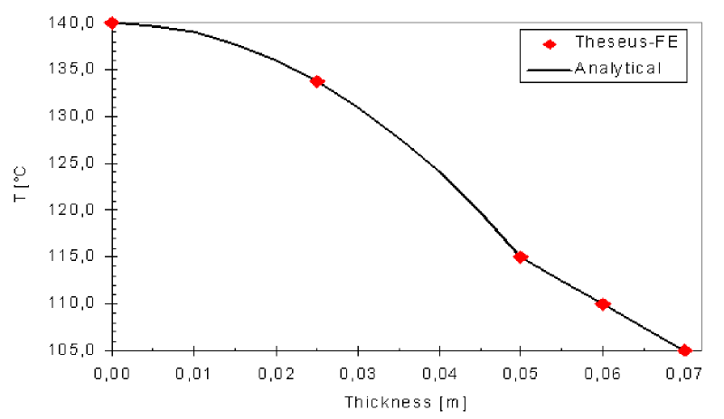
Problem was also modeled with 2 layers and 3 discretization points per layer; results were as accurate as with the higher number of discretization points.
Results
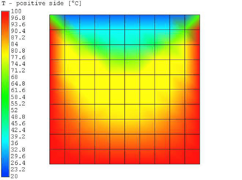
2D conduction in rectangular plate
System
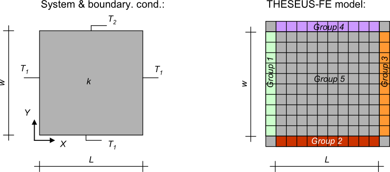
System and boundary conditions
| Quantity | Value | Units | Description |
|---|---|---|---|
| k | 81 | W / m*K | Conductivity |
| L | 0.833 | m | Length |
| w | 0.83 | m | Width |
| T 1 | 100 | °C | Temperature boundary condition |
| T 2 | 20 | °C | Temperature boundary condition |
Problem description
A 2D rectangle is modelled with temperature boundary conditions on all 4 sides. The exact analytic solution is given in [2].
THESEUS‑FE model
12*12 PSHELL3 elements are used to model the rectangle; each with 1 layer and 2 discretization points in the depth direction to represent the and bottom surfaces. The length and width of the FE model are longer than the actual length, to set temperature boundary condition on the faces of groups 1 through 4. Group 5 represents the domain on which temperature is calculated as a function of position.
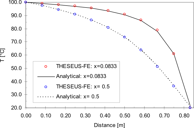
Results
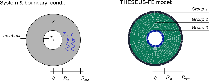
2D conduction in a disk
System
System and boundary conditions
| Quantity | Value | Units | Description |
|---|---|---|---|
| k | 81 | W / m*K | Conductivity |
| R in | 0.065 | m | Inner radius |
| R out | 0.185 | m | Outer radius |
| T 1 | 50 | °C | Temperature on inner edge |
| h | 100 | W / m 2 *K | Convective heat transfer coefficient |
| T ∞ | 20 | °C | Ambiant temperature |
Problem description
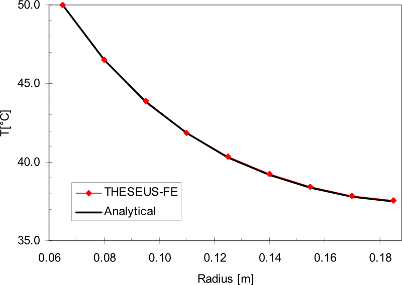
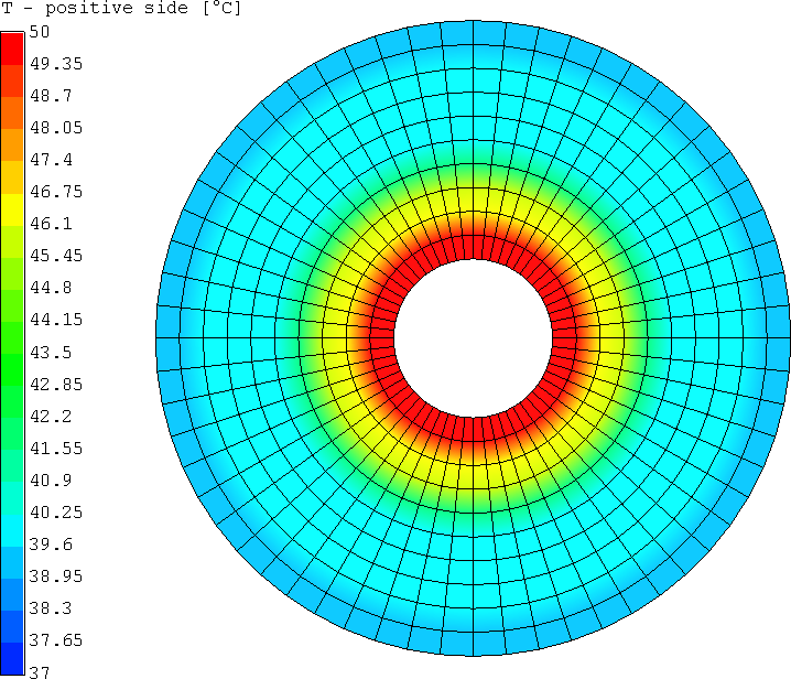
A 2D disk with a hole of radius 0.065m is modelled with temperature boundary condition specified on the inner edge, and adiabatic condition on the outer edge. Convective boundary conditions hold for the rest of the disc. The exact analytic solution is given in [2].
THESEUS‑FE model
3 different groups are used to model the disk, each element is a PSHELL3 with 1 layer and 2 discretization points in the depth direction to represent the and bottom surfaces. The inner and outer radius of the FE model are shorter and longer than the actual lengths, and are used for applying the boundary conditions (group 1 and 3). Group 2 represents the domain on which temperature is calculated as a function of position.
Results
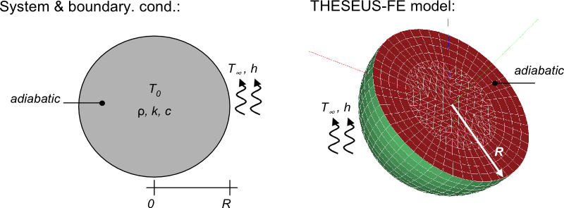
Sphere heating
System
System and boundary conditions
| Quantity | Value | Units | Description |
|---|---|---|---|
| k | 50 | W / m*K | Conductivity |
| ρ | 8000 | kg / m 3 | Density |
| c | 500 | J / kg*K | Heat capacitance |
| R | 0.1 | m | Radius |
| h | 100 | W / m 2 *K | Heat transfer coefficient |
| T ∞ | 100 | °C | Ambiant temperature |
| T 0 | 20 | °C | Initial temperature |
Problem description
A sphere with initial temperature T0 is modeled as it warms to the convective ambient temperature over time. The exact analytic solution is given in [3].
THESEUS‑FE model
Problem was modeled with 3 groups; group 1 is the center face (PSHELL3) where adiabatic boundary condition is applied, group 2 is the outer shell (PSHELL3) where convection is applied and group 3 is the inner solid comprised of HEXA elements.
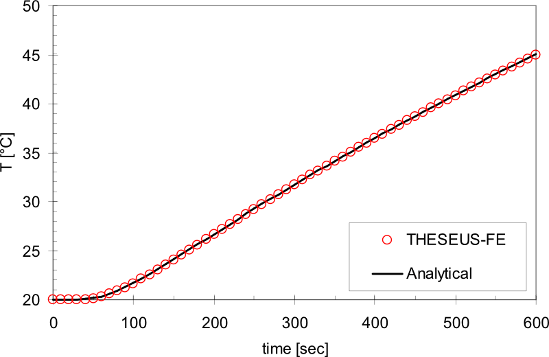
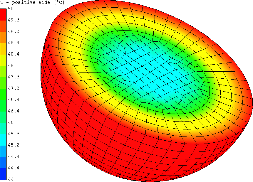
Results
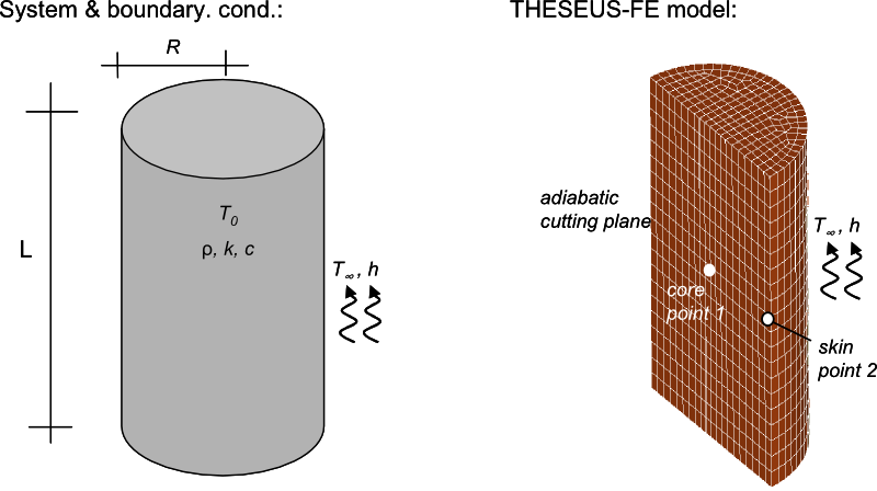
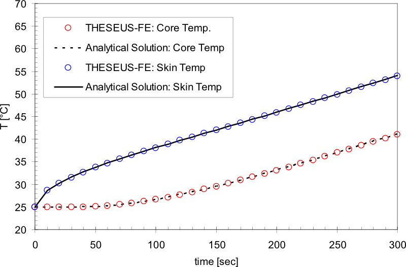
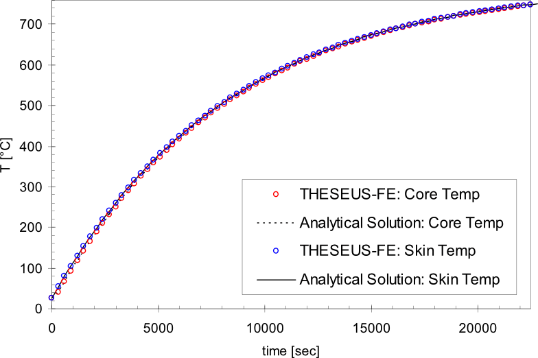
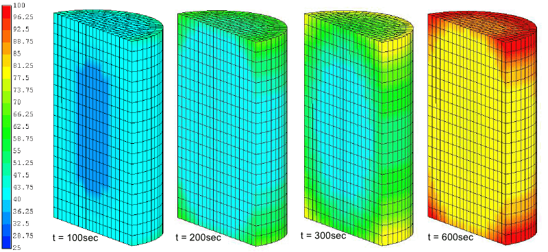
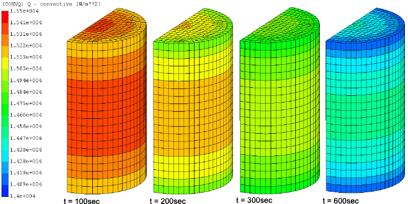
Cylinder heating
System
System and boundary conditions
| Quantity | Value | Units | Description |
|---|---|---|---|
| k | 58 | W / m*K | Conductivity |
| ρ | 8000 | kg / m 3 | Density |
| c | 545 | J / kg*K | Heat capacitance |
| L | 0.3 | m | Length |
| R | 0.1 | m | Radius |
| h | 20 | W / m 2 *K | Convective heat transfer coefficient |
| T ∞ | 800 | °C | Ambient temperature |
| T 0 | 25 | °C | Initial temperature |
Problem description
A cylinder with initial temperature T0 is modeled as it warms to the convective ambient temperature over time. The exact analytic solution is given in [3].
THESEUS‑FE model
Problem was modeled with 3 groups; group 1 is the center face (PSHELL3) where adiabatic boundary condition is applied, group 2 is the outer shell (PSHELL3) where convection is applied and group 3 is the inner solid comprised of HEXA elements.
Results
Infinite body with internal heat impulse
System
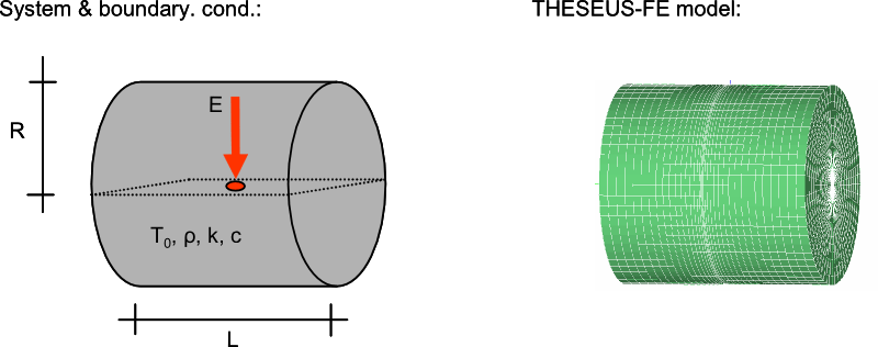
System and boundary conditions
| Quantity | Value | Units | Description |
|---|---|---|---|
| k | 50 | W / m*K | Conductivity |
| ρ | 10000 | kg / m 3 | Density |
| c | 500 | J / kg*K | Heat capacitance |
| L | 0.6 | m | Length |
| R | 0.3 | m | Radius |
| E | 22643.38 | J | Initial energy Input |
| T 0 | 0 | °C | Initial temperature |
Problem description
A cylinder under a Dirac internal heat impulse is modeled. The exact analytic solution is given in [3].
THESEUS‑FE model
The problem was modeled with 2 groups. The heat impulse is applied on group 1, on an internal PSHELL3 mesh of area 2.26E-5 m2 over a time period of 1 second. Group 2 Is a solid element mesh and serves as the body of the cylinder. The cylinder is large enough as to represent an infinite solid for the point load.
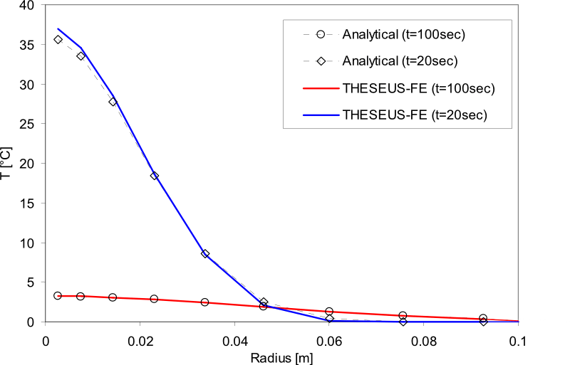
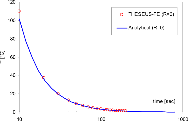
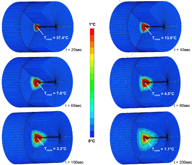
Results
Bibliography
| [1] | INCROPERA, F.P., DEWITT, D.P., Fundamentals of heat and mass transfer, John Wiley & Son, New York, 1996. |
| [2] | MYERS, G.E., Analytical methods in conduction heat transfer, Genium Publishing Corporation, New York, 1987. |
| [3] | BAEHR, H.D, STEPHAN, K., Heat and mass transfer, Springer, Berlin, 1998. |