")
")
Heat bridges
System
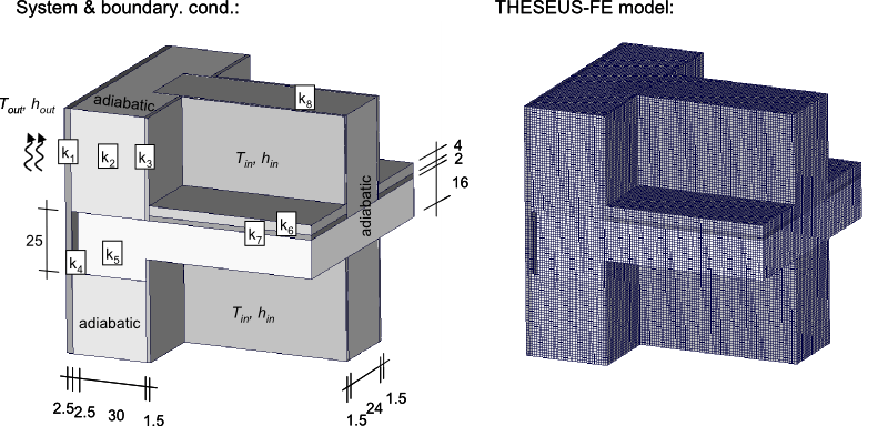
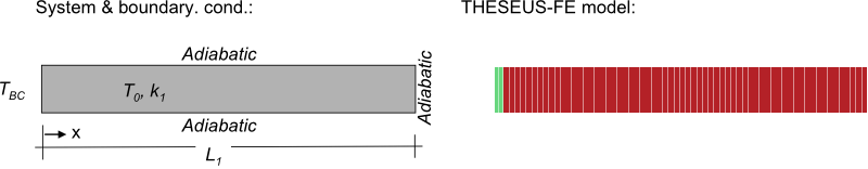
System and boundary conditions
| Quantity | Value | Units | Description |
|---|---|---|---|
| k 1 | 0.87 | W / m*K | Conductivity |
| k 2 | 0.21 | W / m*K | Conductivity |
| k 3 | 0.35 | W / m*K | Conductivity |
| k 4 | 0.093 | W / m*K | Conductivity |
| k 5 | 2.1 | W / m*K | Conductivity |
| k 6 | 1.4 | W / m*K | Conductivity |
| k 7 | 0.04 | W / m*K | Conductivity |
| k 8 | 0.7 | W / m*K | Conductivity |
| T out | 5 | °C | Outside air temperature |
| h out | 25 | W / m 2 *K | Heat transfer coefficient |
| T in | 22 | °C | Inside air temperature |
| h in | 5 | W / m 2 *K | Heat transfer coefficient |
Problem description
Three dimensional heat bridge example, with heat conduction through a composite wall. Convection boundary conditions are assigned on the outer and inner surfaces of the wall. THESEUS‑FE results are compared with experimental results at several corner locations and along edges [1].
THESEUS‑FE model
The problem was modeled with eight groups of solid elements representing the different parts of the composite wall and two groups of PSHELL3 elements. Shell elements are placed on inner and outer surfaces and are used for assigning convection boundary conditions. A uniform mesh with quad elements of approximate length 1cm was used with a total of 390,276 elements.
Results

Anisotropic conductivity
System
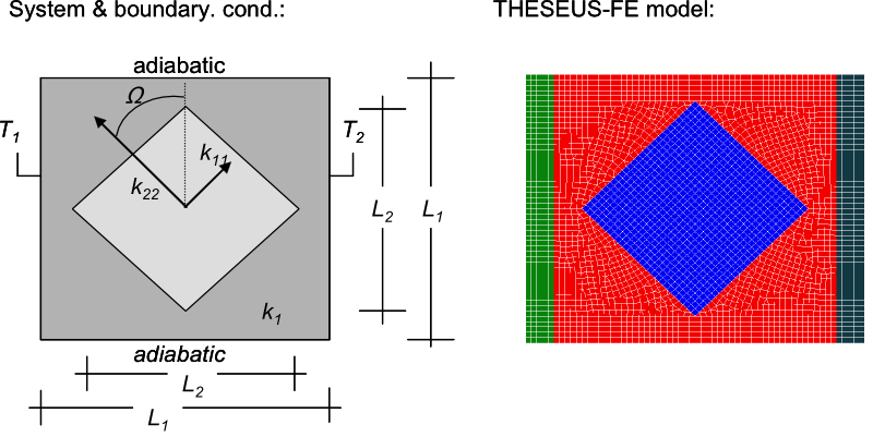
System and boundary conditions
| Quantity | Value | Units | Description |
|---|---|---|---|
| k 1 | 0.56 | W / m*K | Conductivity |
| k 11 | 0.056 | W / m*K | Conductivity |
| k 22 | 0.0056 | W / m*K | Conductivity |
| T 1 | 100 | °C | Temperature boundary condition |
| T 2 | 0 | °C | Temperature boundary condition |
| L 1 | 1 | m | Length |
| L 2 | 0.8 | m | Length |
| Ω | 45 | Degrees | Angle of rotation |
Problem description
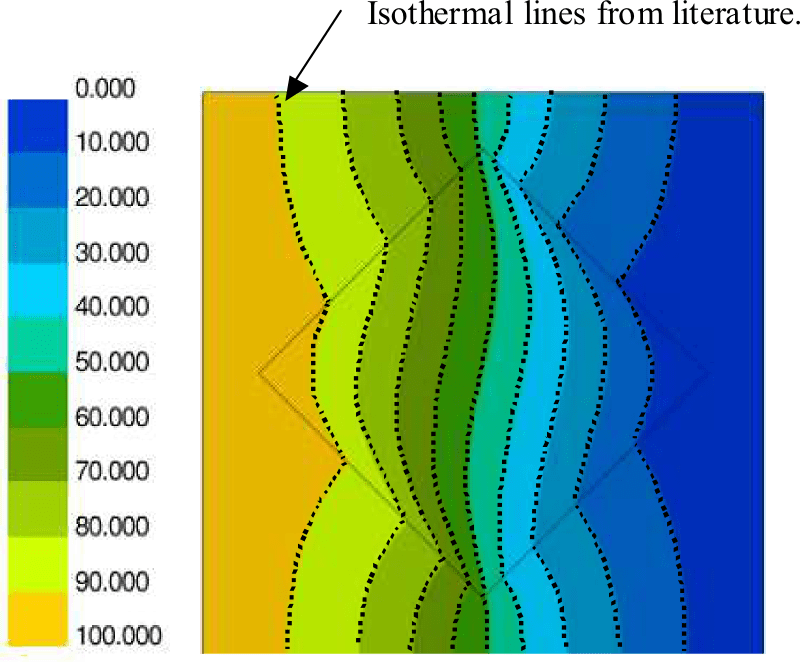
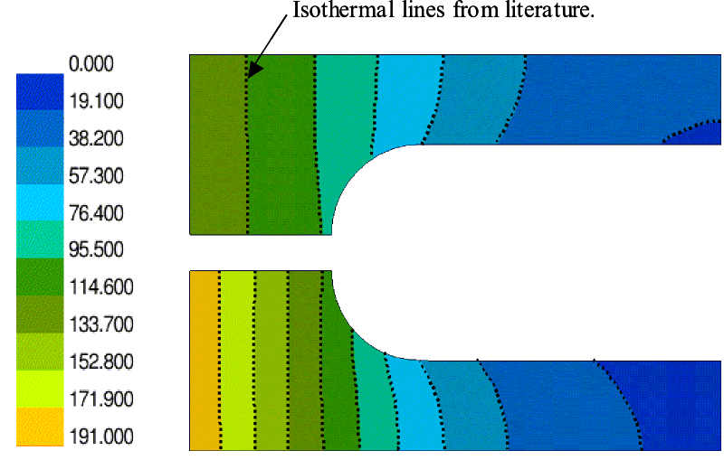
A planar square with a tilted square insert is used to demonstrate the effect of anisotropic conductivity. Referring to Fig. 3, the outer square is an isotropic material with conductivity k1. Constant temperature boundary conditions are imposed on the vertical edges of the square while the horizontal edges are insulated. The inner material is orthotropic with k11 = k1/10 and k22 = k1/100. The orientation of the material axes with respect to the global coordinate axes is 45 degrees. The Fig. 4 shows the temperature field. The distortion of the results due to the anisotropy is clearly visualized. The dotted lines are isothermal lines from literature for validation [2].
THESEUS‑FE model
The problem was modeled with four groups of PSHELL3 elements. Temperature boundary conditions are assigned on the left and right vertical groups. Isotropic material properties are assigned to the outer square while anisotropic material properties are assigned to the local coordinates in tensor form of the inner square.
Results
Temperature dependent conductivity
System
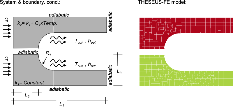
System and boundary conditions
| Quantity | Value | Units | Description |
|---|---|---|---|
| k 1 | 1 | W / m*K | Conductivity |
| C 1 | 0.01 | Constant | |
| T out | 0 | °C | Temperature boundary condition |
| h out | 0.875 | W / m 2 *K | Heat transfer coefficient |
| L 1 | 3 | m | Length |
| L 2 | 0.8 | m | Length |
| L 3 | 1 | m | Length |
| R 1 | 0.5 | m | Radius |
| Q | 100 | W / m 2 | Heat flux |
Problem description
This example illustrates the difference in results when conductivity variations are included in the model. Fig. 5 contains a schematic and mesh for a simple planar geometry. The top and bottom halves are occupied by different isotropic materials; the bottom material has constant conductivity, k1, while the material has a conductivity that varies with temperature as k = k1+C1*T. A constant heat flux is applied along the left edge of the the domain. The right side boundaries are insulated. All other surfaces are convectively cooled with a constant heat transfer coefficient and fluid temperature [2].
THESEUS‑FE model
The problem was modeled with two groups of solid elements of arbitrary thickness and four groups of PSHELL3 elements. Heat flux and heat convection boundary conditions are assigned on the shell elements. Transient 2nd order solver was used with initial time step of 0.1 seconds and a run time of 25 seconds. Variable conductivity is assigned to the second group of solid elements.
Results
Phase change
System
System and boundary conditions
Problem description
| Quantity | Value | Units | Description |
|---|---|---|---|
| k 1 | 1.08 | W / m*K | Conductivity |
| ρ | 1 | kg / m 3 | Density |
| L | 70.26 | J / kg | Latent heat |
| T l | -0.15 | °C | Liqidus temperature |
| T 0 | 0 | °C | Initial temperature |
| T BC | -45 | °C | Temperature boundary condition |
| L 1 | 4 | m | Length |
| t final | 2 | s | Simulation time |
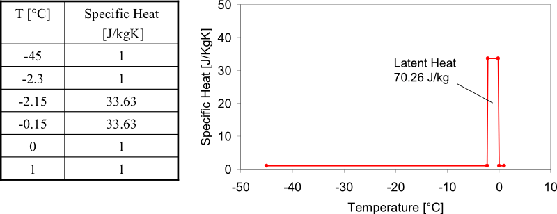
| T [°C] | Specific Heat [J / kgK] |
|---|---|
| -45 | 1 |
| -2.3 | 1 |
| -2.15 | 33.63 |
| -0.15 | 33.63 |
| 0 | 1 |
| 1 | 1 |
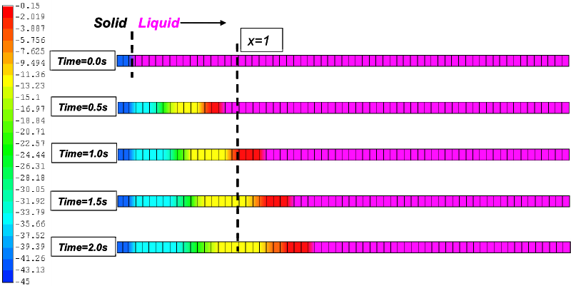
A standard test problem for phase change is the one-dimensional Stefan problem. The problem consists of a material region, with length 4 meters, held initially at a unifrom temperature, T0 = 0°C, that is greater than the liquidus temperature Tl = -0.15°C. At time zero, the left face of the region, x = 0, is lowered to a temperature below the solidus temperature, to TBC = -45°C, causing a solidification front to propagate into the material. All other surfaces are insulated. The schematic of the problem is shown in this Fig. 8[2].
THESEUS‑FE model
The example was solved using 64 PSHELL3 elements in the domain. Temperature boundary conditions are applied on the left hand side and the material specific heat property, was applied via the Tab. 1 shown below. Computation was carried out for a phase change temperature interval of 2 degrees, with solidification starting at -0.15 degrees.
Results
THESEUS‑FE results are compared with the analytical solution. We see a discrepancy of approximately 1 degree, which is attributed to the numerical calculation of the Latent Heat addition. In nature, phase change or Latent Heat addition occurs instantaneously. Numerically, the Dirac impulse function can not be modeled, and therefore we apply the Latent Heat addtion through a 2 degree temperature band. This introduces a modeling error that results in an approximately 1 degree solution error.
Cylinder radiation (open gray-body cavity)
System
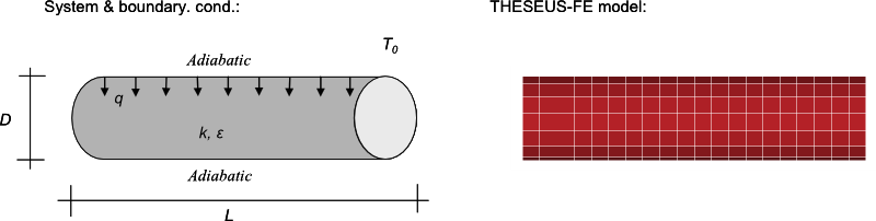
System and boundary conditions
| Quantity | Value | Units | Description |
|---|---|---|---|
| ε | 0.3 | Emission coefficient | |
| k 1 | 1.0 | W / m*K | Conductivity |
| T 0 | 0 | K | Surrounding temperature |
| L | 4 | m | Length |
| D | 1 | m | Diameter |
| q | 200 | W / m 2 | Heat flux |
Problem description
A simple heated enclosure is the circular tube, open at both ends and insulated on the outside surface. For a uniform heat addition q = 200 W / m2 to the inside surface of the tube wall and a surrounding environment at 0 K, we calculate the steady state temperature distribution along the inside surface [3].
THESEUS‑FE model
The open ends of the tube are nonreflecting, and they are assumed to be black bodies at the surrounding temperature 0 K.
In THESEUS‑FE, three major types of radiation heat exchange are realized; for the current problem the model used was open-cavity with gray body radiation.
Gray body radiation considers reflection and absorption of each element and performs a full view factor matrix calculation.
On the inner surface of the cylinder wall, the boundary conditions applied are the background temperature and heat flux.
This is a pure thermal radiation and conduction problem; the material properties assigned are the emission coefficient ε and the conductivity k.
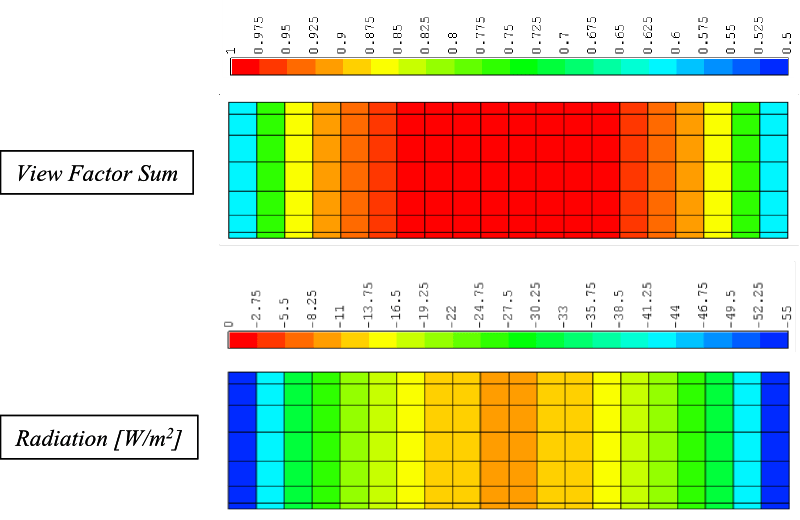
In the images below, the THESEUS‑FE results displayed are the view factor sum of each element, the radiation from each element, and the nodal temperature values.
The view factor is a quantity used to define the fraction of thermal power leaving one element and reaching another.
The sum of the view factor on each element then represents the fraction of thermal power leaving one element and reaching all other elements in the domain.
For enclosed bodies the view factor sum of each element is therefore equal to one.
For open cavities, the value will be less then one, depending on how much thermal power is lost to the environment.
The radiation view factor depends strongly on distance and from the results we can see that thermal power is mainly lost near the cylinder ends, while very little power is lost from elements toward the center of the cylinder. The maximum and minimum view factor sums are 0.975 and 0.6.
The second diagram quantifies how much radiation heat is lost from each element.
For elements near the cylinder ends, it is of magnitude -55 W/m2.
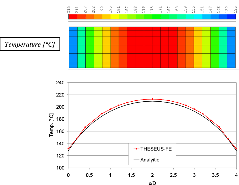
In the last diagram, the temperature results are displayed and compared with the analytic solution.
There is a close agreement between THESEUS‑FE results and the analytic results.
We can further see that there is a 75 degree temperature difference between the center of the cylinder, where little heat is lost compared with elements at the ends of the cylinder where most of the thermal power is lost via radiation.
Results
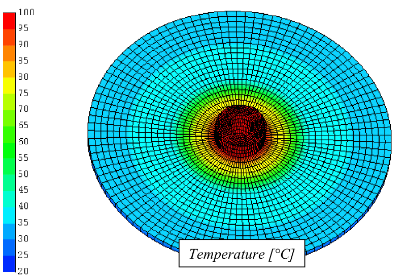
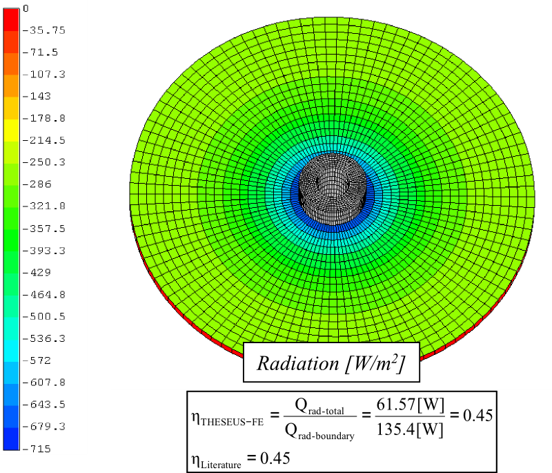
Disk radiation
System
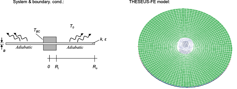
System and boundary conditions
| Quantity | Value | Units | Description |
|---|---|---|---|
| ε | 0.7 | Emission coefficient | |
| k | 15.0 | W / m*K | Conductivity |
| T 0 | -273.15 | °C | Initial temperature |
| T BC | 100 | °C | Boundary condition |
| a | 0.01 | m | Thickness |
| R i | 0.04 | m | Inner radius |
| R 0 | 0.24 | m | Outer radius |
Problem description
An annular fin in vacuum is insulated on one face and around its outside edge. The disk has thickness of 0.01m, inner radius 0.04m, outer radius 0.24m, and thermal conductivity 15.0 W/mK. Energy is supplied to the inner edge from a pipe that fits the central hole and maintains the inner edge at 100 °C. The exposed annular surface, which is diffuse-gray with emissivity 0.7, radiates to the environment at 0 K to investigate performance in a cold environment. Results are shown for the temperature distribution as a function of radial position along the disk, the radiation flux from each element and the radiation efficiency of the disk calculated from THESEUS‑FE is compared with results from literature [3].
THESEUS‑FE model
The disk is assumed thin enough so that the local temperature is considered constant across the thickness. For surroundings at zero temperature there is no incoming radation. Temperature boundary condition is specified at the inner radius of the fin and adiabatic conditions are specified on the bottom and outer edge of the fin. The total number of elements is 4284. The problem was calculated as a transient problem for 6 seconds, at which time steady state was reached.
Results
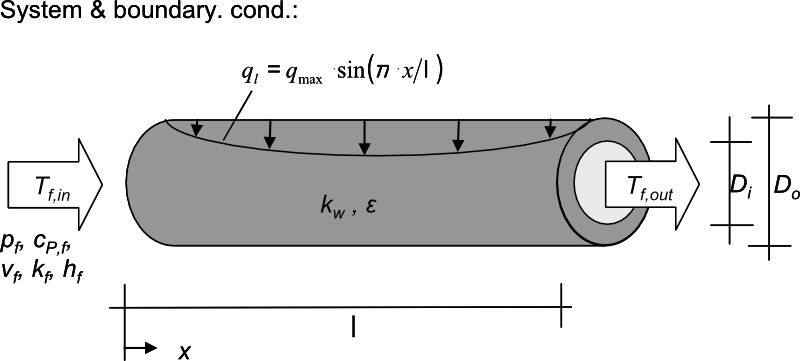
Cylinder Radiation with 1D flow
System
System and boundary conditions
| Quantity | Value | Units | Description |
|---|---|---|---|
| k w | 24.0 | W / mK | Wall conductivity |
| ε | 1 | Wall emisivity | |
| ρ f | 2 | kg / m 3 | Fluid density |
| c p,f | 1 | kJ / kg*K | Fluid specifik heat |
| k f | 0.044 | W / m*K | Fluid conductivity |
| v f | 5E-5 | m / s | Fluid inlet velocity |
| h f | 3.4 | W / m 2 K | Fluid convective heat transfer coefficient |
| T f,1 | 357 | °C | Fluid inlet temperature |
| q max | 1750 | W / m 2 | Maximum applied heat flux density |
| l | 1 | m 2 K | Tube length |
| D o | 0.052 | m | Tube outer diameter |
| D i | 0.048 | m | Tube inner diameter |
Problem description
A fluid with inlet temperature 357°C flows through a 1m long circular tube with inner and outer diamter 0.048m and 0.052m respectivly.
The convective heat transfer coefficient is calculated based on a laminar flow assumption throughout the tube.
The Reynolds number of the flow is 672 which is well below the transition region of 2100-4000.
The Nusselt number for a pipe with laminar flow is then constant, and the convective heat transfer coefficient is also constant.
The tube outer surface is perfectly insulated while the inner surface is heated electrically with a sinusoidal heat flux of maximum value 1750 W/m2.
The inner wall of the tube is considered as a black body, and heat radiation from element to element and element ot environment is accounted for.
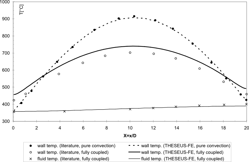
In this problem we consider the combined effects of convection, conduction and thermal radiation, and compare temperatue results for the wall and the fluid along the axial direction with results from literature.
The schematic of the problem is shown in this Fig. 17[3].
THESEUS‑FE model
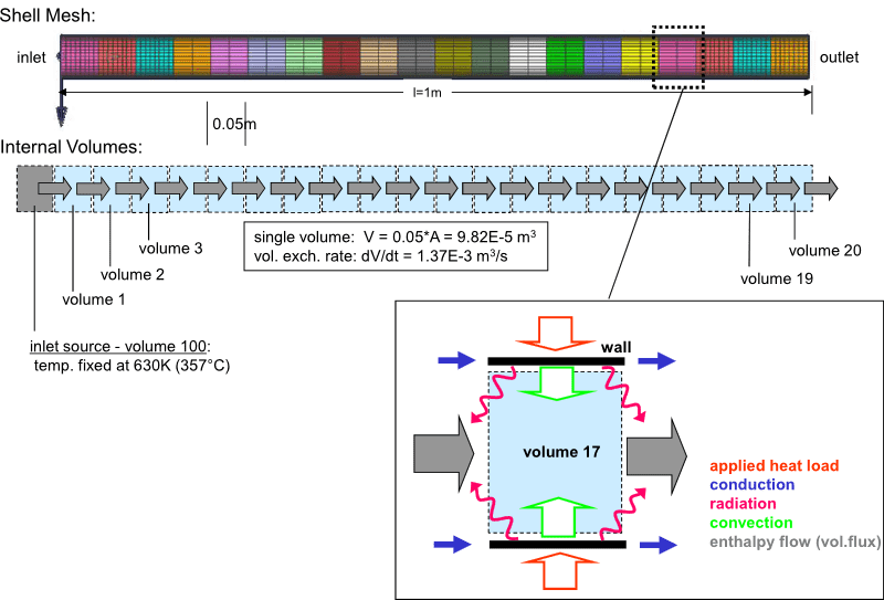
THESEUS‑FE model contains 3115 quad PSHELL1 elements of thicknes 0.002m. The domain is divided into 20 'volumes' plus one source volume on which the inlet flow conditions are specified. A 'volume' in THESEUS‑FE is a bounded areas with one degree of freedom, Tvol, that is spatially constant throughout the volume. Finite elements and volumes are coupled via convection. We consider the wall to be a black body (emissivity=1), that absorbes all incoming energy. For the background (environment) radiation temperature, the specified inlet flow temperature and the calculated outlet flow temperature are used. After the outflow temperature is calculated, the radiation background temperature is updated and the calculation is rerun. This procedure is carried out until convergence in outflow temperature is reached. Within each volume element, the combined effects of convection from the fluid, conduction within the wall and heat radiation from the wall to the environment and to other elements, determines the wall and fluid temperature. In this Fig. 18 the interplay of these phenomona are visually shown. The problem is calculated as a steady state problem.
Results
In Fig. 19 we compare THESEUS‑FE temperature results along the tube length with that from literature.
We can see that the fluid temperature for the fully coupled problem (radiation, conduction and convection) closely meets with results from literature.
For the wall temperature, results are shown for the fully coupled problem and for the pure convection problem, ignoring radiation and conduction.
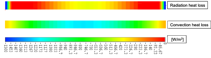
To conduct a further analysis of the problem, in the Fig. 20 we compare heat loss through radation and heat loss through convection from each element.
Near the inlet and outlet of the tube, heat loss is strongly driven by radiation while through the center of the tube convection dominates.
Bibliography
| [1] | HAUSE G., STIEGEL H. "Wärmebrücken Atlas für den Mauerwerksbau", Baueverlag. |
| [2] | REDDY, J.N., GARTLING, D.K. The Finite Element Method in Heat Transfer and Fluid Dynamics 2nd Edition. Boca Raton: CRC Press LLC, 2000. |
| [3] | SIEGEL R., HOWELL J.R. 2002, "Thermal Radiation Heat Transfer", 4th Edition, Taylor & Francis. |